Automatic Calibration For Machine Learning

If a machine learning model is trained on simulated data, then it will likely need to be corrected for differences between that training data (“simulation”) and data collected from experiment (“data”). It may also be necessary to introduce variations to simulated data that reflect uncertainties in how the simulation is performed or the values of underlying physical constants.

At the ATLAS experiment studying proton-proton collisions at CERN, particle identification models are trained on simulation and then calibrated to agree with data. This involves deriving scale factors that weight individual collisions so that distributions between simulation and data agree. The previously mentioned variations then appear as uncertainties on those scale factors, which reflect the difference in model output between the nominal training data and variations. If a model can be trained to reduce this difference in model outputs, then it will also have smaller final uncertainties and therefore better predictive power. This article wil demonstrate how this can be done with a toy example employing a special loss function.

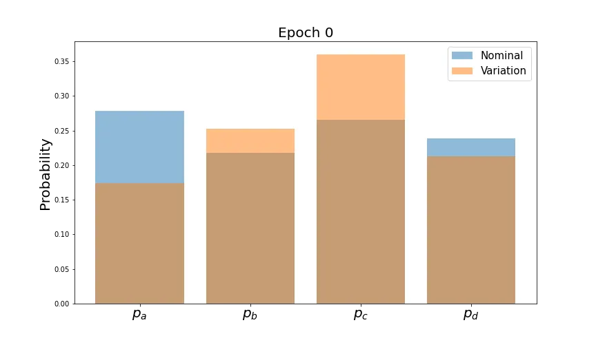
First, let’s create a mock dataset on which to train our model. We will sample from a 10-dimensional Gaussian which will be centered at 0 and with variance of 1 in all dimensions. This will serve as our “nominal” dataset. We will also create another, our “variation” dataset, that is identical save for instead being centered at (2,2,2,..) in all dimensions. We’ll generate 2048 of these samples.

N_DIM     = 10
N_SAMPLES = 2048
N_CLASSES = 4
xa = torch.randn(N_SAMPLES, INPUT_DIM)
xb = torch.randn(N_SAMPLES, INPUT_DIM) + 2.0

Next let’s create a very simple neural network classifier model that takes in our 10 input features and predicts a four-class output. As a concrete example, this might classify a building as a store, highrise, single-family home, or office based on various features like square footage, number of floors, etc. Our model will be feedforward network with two hidden layers of 16 neurons each with ReLU between layers and Adam as our optimizer. These details of the architecture are not particularly import for our problem.

class TinyClassifier(nn.Module):
    def __init__(self):
        super().__init__()
        self.net = nn.Sequential(
            nn.Linear(INPUT_DIM, HIDDEN_DIM),
            nn.ReLU(),
            nn.Linear(HIDDEN_DIM, N_CLASSES),
        )

    def forward(self, x):
        return self.net(x)

model = TinyClassifier().to(DEVICE)
opt   = torch.optim.Adam(model.parameters(), lr=LR)

While this is a classifier model, we are not going to give it a loss based on classification label as this would make it difficult to disentangle it from our real object of study. Instead, we are going to add a loss term based on the difference in model outputs between our nominal and variation datasets. We’ll look at two different ways to calculate this difference, which both measure the difference in output distribution between datasets.

Kullback-Leibler (KL) Divergence

This metric, also called the relative entropy, measures the difference between two probability distributions. Its definition is:

$$D_\text{KL}(P||Q) = \sum_{x \in X}P(x)\log\frac{P(x)}{Q(x)}$$

You may notice that this definition is asymmetric in $P(x)$ and $Q(x)$. We can define a symmetric metric then as the following:

$$D_\text{KL} = \frac{1}{2}[D_\text{KL}(P||Q) + D_\text{KL}(Q||P)]$$

Because the KL Divergence requires probability distributions, it will take as input the set of mean probability predictions for our 4 output classes over an entire batch.

# Forward
logits_a = model(xa_batch)
logits_b = model(xb_batch)

# Two‑way (symmetrised) KL
log_pa   = F.log_softmax(logits_a, dim=1).mean(dim=0)   # log‑probs (input)
pa       = log_pa.exp()                     # probs
log_pb   = F.log_softmax(logits_b, dim=1).mean(dim=0)
pb       = log_pb.exp()
loss_ab  = F.kl_div(log_pa, pb, reduction="batchmean")
loss_ba  = F.kl_div(log_pb, pa, reduction="batchmean")
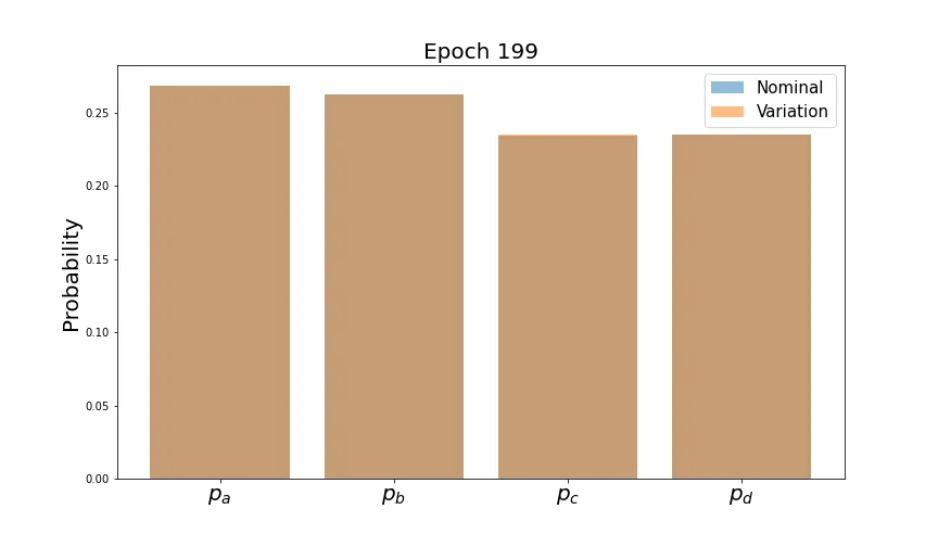
syst_loss     = 0.5 * (loss_ab + loss_ba)

Let’s train with this loss function and see how the mean predictions look at the beginning and end.

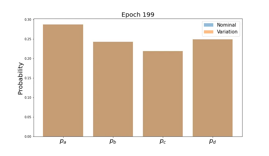
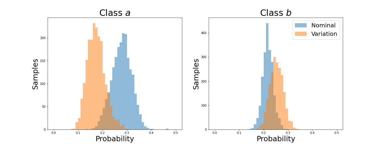
As desired, the predictions line up very well by the end of training. However, we’d like the distributions of each probability to converge. Let’s plot these and see how they evolve for the first two classes (the behavior is similar for the others).

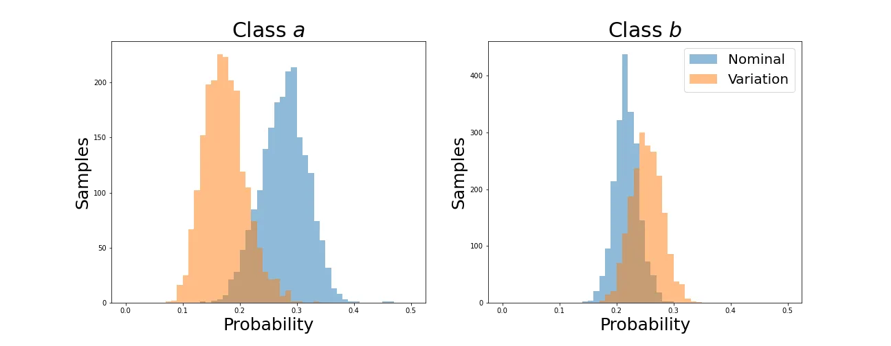
You can see that indeed the means converge as shown in the four-class plots. The problem is that this is accomplished by collapsing the distributions down to spikes around a single value. This would be disastrous for any other task that we wanted this network to learn, so let’s see if it can be avoided.

Wasserstein Distance

This metric represents the amount that a distribution must be redistributed to transform the initial into the final. It is also known as the Earth-Mover’s Distance, evoking the original inspiration of measuring the total effort to move a pile of earth into another some distance. This can be calculated using two simple lists of values. In 1-D, the calculation involves sorting each list and finding the distance between values at identical indices.

loss = 0
for class_i in range(N_CLASSES):
    pa1 = F.softmax(logits_a, dim=1)[:, class_i]     # shape (B,)
    pb1 = F.softmax(logits_b, dim=1)[:, class_i]
    # 1‑Wasserstein distance between two 1‑D empirical distributions:
    pa1_sorted, _ = pa1.sort()         # differentiable in PyTorch ≥1.8
    pb1_sorted, _ = pb1.sort()
    loss += torch.mean(torch.abs(pa1_sorted - pb1_sorted))

Here we are calculating the Wasserstein Distance between the predicted probabilities for a single class. We must then loop over all outputs classes, calculating a distance for each and summing them all. This gets us closer to true alignment of model outputs than training to minimize on the mean of 4-class probabilties over an entire batch as we do with the KL Divergence above.

Let’s first verify that this has the expected behavior on the output probabilities.

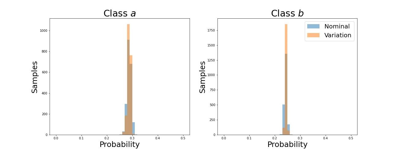
As before, average values converge. Now let’s see how the individual distributions evolve.

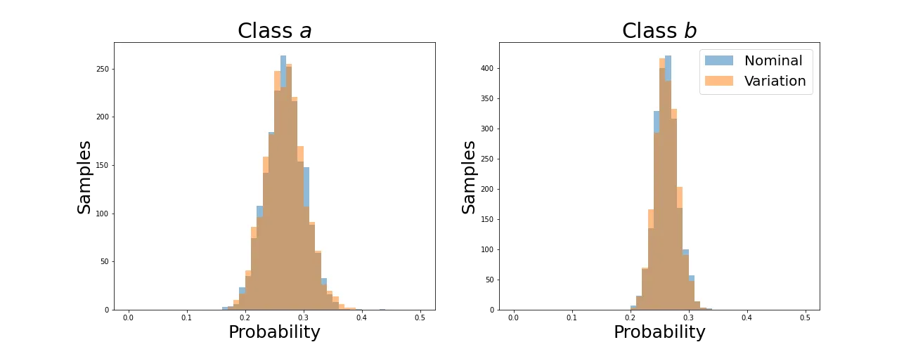
We can see that the distributions retain their shapes instead of collapsing to a spike as with the KL divergence. This is because the Wasserstein Distance is not simply aligning averages but individual values for each sample.

Conclusion

We’ve explored two different methods for aligning the outputs of a network across two different samples. Of these, the Wasserstein Distance allowed for a more comprehensive alignment as implemented. Our toy example used only these loss terms, but a real network will of course have some other primary task. We’ll explore next how our network behaves when this is added.

You can see the full code for training the above models at this Gist.